A probabilistic electrical simulator
Jonas Bodingbauer
February 01, 2024
Electrical Circuit: Voltage divider
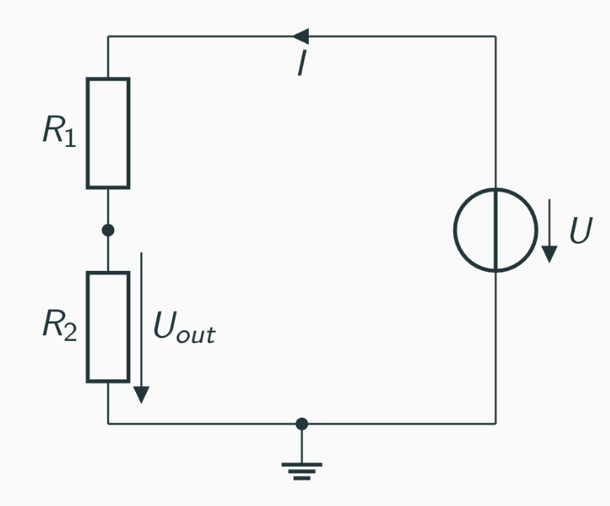
\[U_{out} = U \frac{R_2}{R_1 + R_2}\]
Idea
- Components in a circuit have an expected value and a tolerance.
- Circuit gets input and produces a response.
- The response is a random variable described by a probability distribution.
- Priors and Observed are linked by the simulator model.
- Additional randomness: device noise, instrument noise, offsets, ...
Electrical Simulations
- DC Analysis
- AC Analysis (treat everything as a linear component)
- DC Analysis with nonlinearity (e.g. diodes)
- Transient Analysis
- Lots more...
Finally, some modelling!
\[ \underbrace{\begin{bmatrix} \mathbf{Y'} & \mathbf{B}\\ \mathbf{C} & \mathbf{D} \end{bmatrix}}_{Y} \cdot \underbrace{\begin{bmatrix} \vec{\varphi}\\ \vec{I} \end{bmatrix}}_{x} = \underbrace{\begin{bmatrix} \vec{J}\\ \vec{E} \end{bmatrix}}_{F} \]
AC-Case: Domain changes to complex numbers (Fourier transform)
Nonlinear case: Newton-Raphson fixed-point iteration
\[ \mathbf{Y}(\vec{x}_i) \cdot \vec{x}_{i+1} = -\mathbf{F}(\vec{x}_i) + \mathbf{Y}(\vec{x}_i) \cdot \vec{x}_i \]
Program flow
- Read SPICE-like file
voltagediv.cir
V1 0 in DC 2
R3 in 2 11.72
R1 2 3 1.2k
R2 3 0 1.8k
voltagediv.tol
R3 0.1%
R1 5%
R2 5%
- Determine the matrix size
- Read observed data from file(s)
- Run inference using the simulator as a model
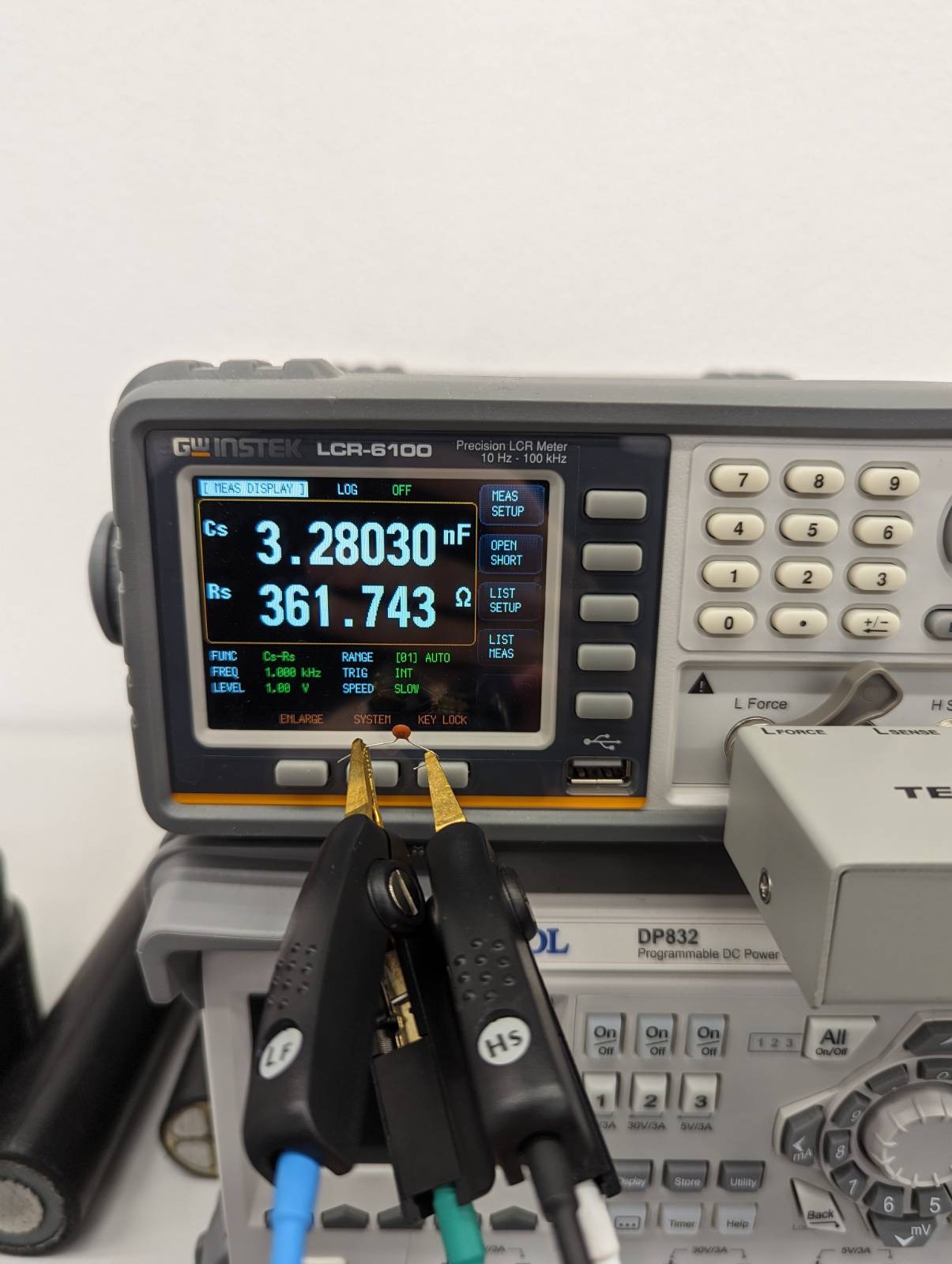
Measurements
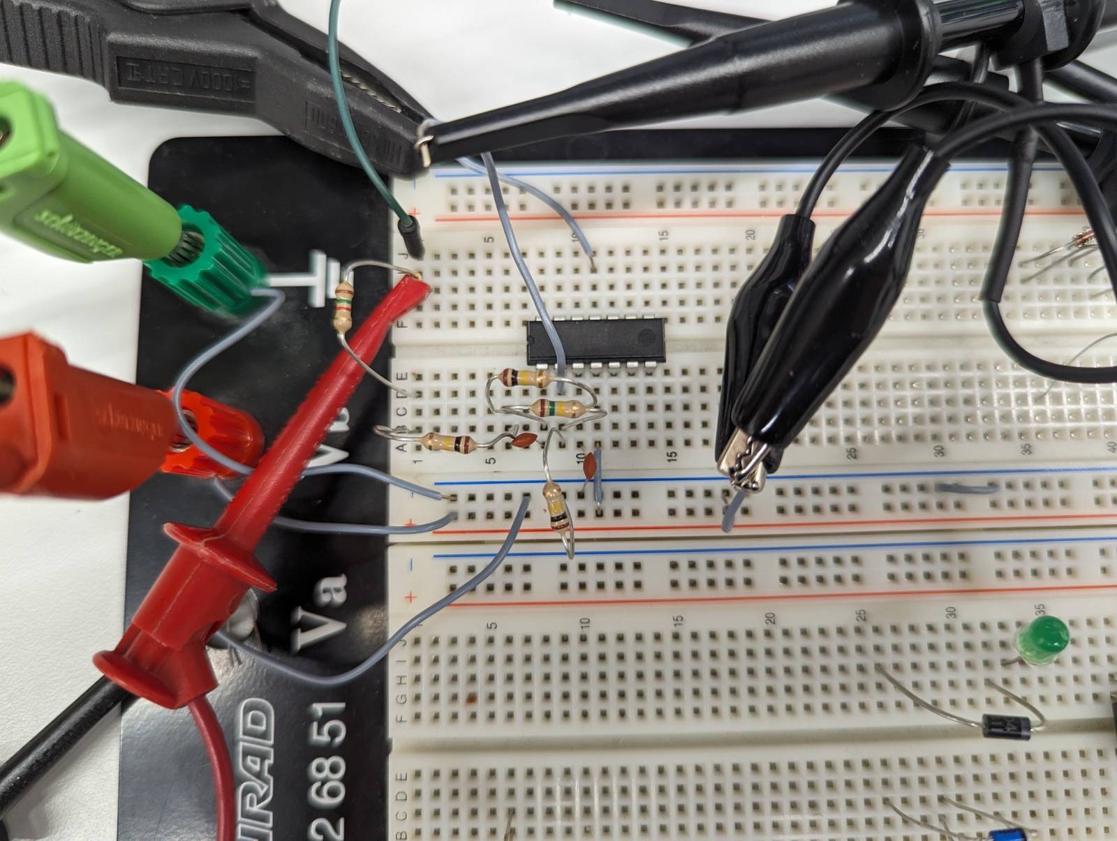
First example extended
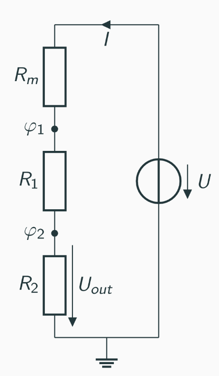
- \(R_m\) is an additional precision resistor for measuring current.
- \(\varphi_1\) and \(\varphi_2\) are potentials.
- Priors:
\(R_1\), \(R_2\) normally distributed around nominal value.\(U_{offset_1}\), \(U_{offset_2}\) normally distributed around 0.\(U_{noise_1}\), \(U_{noise_2}\) uniformly distributed in \([0, 0.1]V\).
- Observed: \(\varphi_1\), \(\varphi_2\)
Results

Glorified linear regression?

Glorified linear regression?

Glorified linear regression?

Glorified linear regression?
| Component | Nominal Value | "True" Value | MAP-Estimate |
|---|---|---|---|
| \(R_1\) | \(1.2\,\text{k}\Omega\) | \(1.176\,\text{k}\Omega\) | \(1.186\,\text{k}\Omega\) |
| \(R_2\) | \(1.8\,\text{k}\Omega\) | \(1.784\,\text{k}\Omega\) | \(1.776\,\text{k}\Omega\) |
| \(R_3\) | \(11.72\Omega\) | \(11.72\Omega\) | \(11.72\Omega\) |
| \(U_{offset_1}\) | ? | ? | \(-0.059\text{V}\) |
| \(U_{offset_2}\) | ? | ? | \(-0.026\text{V}\) |
| \(U_{noise_1}\) | ? | ? | \(0.2\,m\text{V}\) |
| \(U_{noise_2}\) | ? | ? | \(10^{-5}\text{V}\) |
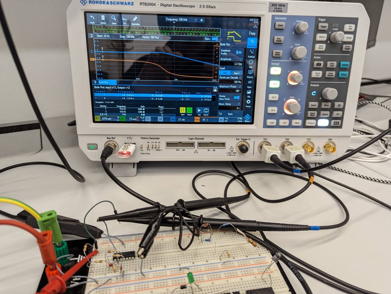
A more complex circuit
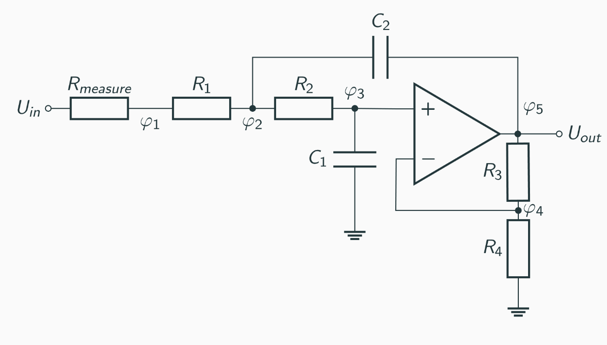
Frequency Response


Results
Obtained with three measured potentials: \(\varphi_1\), \(\varphi_2\), \(\varphi_5\).
| Component | Nominal Value | "True" Value | MAP-Estimate |
|---|---|---|---|
| \(R_1\) | \(100\,\text{k}\Omega\) | \(100.09\,\text{k}\Omega\) | \(100.08\,\text{k}\Omega\) |
| \(R_2\) | \(100\,\text{k}\Omega\) | \(99.97\,\text{k}\Omega\) | \(98.6\,\text{k}\Omega\) |
| \(R_3\) | \(150\,\text{k}\Omega\) | \(149.5\,\text{k}\Omega\) | \(151.2\,\text{k}\Omega\) |
| \(R_4\) | \(100\,\text{k}\Omega\) | \(100.06\,\text{k}\Omega\) | \(99.19\Omega\) |
| \(C_1\) | \(3.3\,\text{nF}\) | \(2.75\,\text{nF}\) | \(2.73\,\text{nF}\) |
| \(C_2\) | \(3.3\,\text{nF}\) | \(3.33\,\text{nF}\) | \(3.32\,\text{nF}\) |
Inference
- Turing NUTS sampler performs really well.
- Also tried other samplers (SMC, PG, Gibbs), but they did not work reasonably well without further tuning.
- ADVI works wonders for this application (MAP estimate in seconds).
- Choice of priors is important: output often depends on a ratio of variables, so scaled variables may be equally likely.
Normal distributed priors
Uniform priors

Challenges
- Getting Automatic Differentiation to work was quite a hassle (types...).
- Big range of values (e.g. \(10^{-12} - 10^{6}\)) does not play nicely with NUTS.
- Fixed by scaling variables and using logarithmic frequency response.
- Hard to know if results are actually reasonable if you do not know the true values.
Conclusion
- It works!
- Modelling needs to account for many effects to be realistic (measurement offsets, noise, parasitics, ...).
- The nonlinear system suffers from convergence issues with some parameters explored by inference.
- More components: transistors (BJT, MOSFETs, ...).
- Transient analysis.
Thank you for your attention!
Questions?

Nonlinear Diode

DC Analysis Model
@model function dcanalysis(...)
  for e in keys(tolerances) ...
      elementsR[e].R ~ Normal(elements[e].R,
                  elements[e].R * tolerances[e])
  end
  offsets ~ MvNormal(zeros(observedNodeIndicesLength),
                    diagm(0.01 .* ones(observedNodeIndicesLength)))
  for i in 1:observedNodeIndicesLength
      noise[i] ~ Uniform(0, 0.01)
  end
  A,RHS = assembleMatrixAndRhs(elementsR,nodes,type)
  Ainv = inv(A)
  for i in 1:amountOfMeasurements
      RHS[nodes[elementsR["V1"].name]-1] = -voltages[i]
      res = Ainv * RHS
      results[i,:] = res[observedNodeIndices]
  end
  for (i,col) in enumerate(eachcol(results))
      measurementMatrix[:,i] ~ MvNormal(col .+ offsets[i],
              diagm(noise[i] * ones(amountOfMeasurements)))
  end
end
Sallen Key Input
V1 0 in AC 1
R5 in 1 1.484k
R1 1 2 100k
R2 2 3 100k
C1 2 out 3.3n
C2 3 0 3.3n
R3 out 4 150k
R4 4 0 100k
O1 3 4 out 0 1e5
R5 0.001%
R1 0.5%
R2 0.5%
R3 0.5%
R4 0.5%
C1 40%
C2 40%
Sallen Key Measurements
in Sa,Frequency in Hz,Gain in dB,Phase in deg,Amplitude in Vpp
1.00E+00,1.000E+01,-2.426E-02,2.693E-03,2.500E+00
2.00E+00,1.023E+01,-2.448E-02,3.685E-03,2.500E+00
3.00E+00,1.047E+01,-2.481E-02,6.256E-04,2.500E+00
4.00E+00,1.072E+01,-2.359E-02,1.049E-02,2.500E+00
5.00E+00,1.096E+01,-2.475E-02,1.010E-02,2.500E+00
6.00E+00,1.122E+01,-2.326E-02,4.135E-03,2.500E+00
7.00E+00,1.148E+01,-2.272E-02,1.164E-02,2.500E+00
8.00E+00,1.175E+01,-2.387E-02,-7.126E-03,2.500E+00
9.00E+00,1.202E+01,-2.171E-02,1.350E-03,2.500E+00
...